The Fair Price to Pay a Spy: An Introduction to the Value of Information

Spy image

(This article covers the decision-theoretic concept of value of information through a classic example.)

What is the value of a piece of information?

It depends. Two factors determine the value of information: first, whether the information is new to you; second, whether the information causes you to change your decisions.

The first point is immediately clear as you would be unwilling to pay a reward for information which you already know. Information is understood here in the sense of probabilistic knowledge represented by a probability distribution. As such, if the information keeps your beliefs unchanged, it cannot have any value.

The second point is more subtle. Only decisions and actions can have value, information itself has only indirect value through the decisions and actions that it influences. The consequence of a decision is a realized utility which can be both positive or negative. As a simple monetary example, imagine you buy a share of a company. Then the utility is a function of the change in the share price. Information such as insider information can lead to a belief that the share price will drop, thus leading to the decision to sell the share and realize the utility. If the information I learn about the company does not change my decision whether to sell the share or not, then it also cannot change the utility. Therefore value is understood as a subjective but quantitative utility that is realized at decision time.

The Fair Price to Pay a Spy

The following example is from one of the important papers on decision theory and decision analysis, now in its 50th anniversary year(!), (Howard, "Information Value Theory", 1966). Unfortunately the paper is behind a paywall, but I will keep the presentation below self-contained and also took the liberty to update the exotic notation used in the paper to a more modern form.

Imagine you run a construction company and the government advertises a contract to build a large development. The bidding happens via a lowest price closed bidding, where every construction company submits a price for which they would construct the development in a technically acceptable manner. You do not see any competing bids and the lowest-price bid wins.

Leaving moral and legal concerns aside, how much would you pay a spy to reveal to you the lowest competing bid prior to you making your bid? We will follow Ronald Howard in answering this question using decision theory, thus putting a monetary value on a piece of information.

The following are the key quantities in this problem:

$E$, the expense to your company in constructing the development. It is a random variable.
$L$, the lowest price among all competing bids. It is a random variable.
$B$, your bid. It is a decision variable under your control, not a random variable.
$V$, the profit you realize, a random variable.

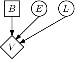
The situation is represented using influence diagrams in the following figure. (Incidentally influence diagrams were also first formally published by Ronald Howard in (Howard and Matheson, "Influence diagrams", 1981), and a nice historical piece on them is available from Judea Pearl in (Pearl, "Influence Diagrams - Historical and Personal Perspectives", 2005).)

Influence diagram for the construction company

In the diagram the round nodes represent random variables, just like in directed graphical models (Bayesian networks). The rectangular node represents a decision node under our control, here the bid $B$ we submit. The diamond shaped utility node represents a value achieved, in our case the profit $V$. The above diagram is not enough, we need to specify how our profit $V$ comes about.

The first step in applying decision theory is to assume that everything is known. So let us assume $B$, $E$, $L$ are known. Then, it is easy to see whether we actually won the contract, i.e. whether our bid is small enough, $B < L$. If $B \geq L$, we do not obtain the contract and the profit is zero. (We assume here, for simplicity, that the cost for making the bid is zero.) If we won the bid, that is, if $B < L$ is true, then the profit is simply the bid price minus our expenses, $B - E$. Therefore we have the profit as a function of $B$, $E$, and $L$ as

$$V = \left\{\begin{array}{cl}0,&\textrm{if $B \geq L$,}\\ B-E,&\textrm{if $B < L$.}\end{array}\right.$$

The above expression can also be written using indicator notation as $V = \mathbb{1}_{\{B < L\}} \cdot (B-E)$.

But $B$, $E$, $L$ are not known. The second step in applying decision theory is therefore to take expectations with respect to everything that is unknown ($E$ and $L$ in our case) and to maximize utility with respect to all decisions ($B$ in our case). We do this in two steps. Let us first assume $B$ is fixed. Then we take the expectation of the above expression with respect to the unknown $E$ and $L$,

$$\mathbb{E}[V | B] = \mathbb{E}_{E,L}[\mathbb{1}_{\{B < L\}} \cdot (B-E)].$$

Now we further assume independence of the cost $E$ and the lowest competing bid $L$, that is $P(E,L) = P(E) \, P(L)$, a reasonable assumption. Here is an example visualization of priors $P(E) = \textrm{Gamma}(\textrm{Shape}=80,\textrm{Scale}=6)$ and $P(L) = \mathcal{N}(\mu=1100, \sigma=120)$.

Priors of cost and lowest bid

Assuming independence we obtain

\begin{eqnarray} \mathbb{E}[V | B] & = & \mathbb{E}_{E,L}[\mathbb{1}_{\{B < L\}} \cdot (B-E)]\nonumber\\ & = & P(B < L) (B - \mathbb{E}_E[E]).\label{eqn:VgivenB} \end{eqnarray}

The expression (\ref{eqn:VgivenB}) is intuitive: the expected profit is given by the probability of winning the bidding times the difference between bid and expected cost. Here is a visualization for the above priors, with our bid $B$ on the horizontal axis.

Expected profit as a function of our bid

You can see three regimes: 1. When $P(B < L)$ is very large (up to about $B=850$) the expected profit behaves linearly as $B-\mathbb{E}_E[E]$, and if we bid below our actual cost we realize a negative profit (loss). 2. When $P(B < L)$ is very small (above $B=1300$) the expected profit drops to zero. 3. Between $B=850$ and $B=1300$ we see the product expression resulting in a nonlinear profit as a function of B.

To finish the second step of applying decision theory we have to maximize (\ref{eqn:VgivenB}) over our decision $B$, yielding

$$\mathbb{E}[V] = \max_{B} \mathbb{E}[V|B].$$

This tells us how to bid without the help of a spy: in the above example figures, we obtain an expected profit $\mathbb{E}[V] = 421.8$ for a bid of $B=966.2$.

Revealing $L$ gives a large competitive advantage, but how much would we be willing to pay a spy for this information? To this end Howard introduces the concept of clairvoyance and value of information.

In clairvoyance we consider what could happen if a clairvoyant appears and offers us perfect information about $L$. If we would know $L$ we can compute as before

\begin{eqnarray} \mathbb{E}[V | B, L] & = & P(B < L) (B - \mathbb{E}_E[E])\nonumber\\ & = & \mathbb{1}_{\{B < L\}} (B - \mathbb{E}_E[E]),\nonumber \end{eqnarray}

where the probability $P(B < L)$ is now deterministic one or zero as $B$ is our decision and $L$ is known. As $B$ is our decision we again maximize over it.

\begin{eqnarray} \mathbb{E}[V | L] & = & \max_B \mathbb{E}[V | B,L]\nonumber\\ & = & \max_B \mathbb{1}_{\{B < L\}} (B - \mathbb{E}_E[E])\nonumber\\ & = & \left\{\begin{array}{cl}L - \mathbb{E}_E[E], & \textrm{if $L > \mathbb{E}_E[E]$,}\\ 0, & \textrm{otherwise (do not bid).}\end{array}\right.\nonumber \end{eqnarray}

The last step can be seen as follows: our bid $B$ should be above our expected expenses $\mathbb{E}_E[E]$ otherwise we would incur a negative profit but $B$ should also be as high as possible just below $L$. Hence if this is impossible ($L \leq \mathbb{E}_E[E]$) we do not bid. Otherwise we bid $B=L-\epsilon$ and realize the expected profit $L-\mathbb{E}_E[E]$.

Ok, so this tells us how to bid when we know $L$. But we do not know $L$ yet. Instead we would like to put a value on the information about $L$. We do this by integrating out $L$,

$$\mathbb{E}_L[\mathbb{E}[V|L]]$$

(Howard introduces a special notation for the above expression, but I am not a fan of it and will omit it here.)

The value of information (value of $L$) is now defined as

$$\textrm{EVPI}(L) = \mathbb{E}_L[\mathbb{E}[V|L]] - \mathbb{E}[V].$$

This quantity is again intuitive: the value of knowing $L$ is the expected difference between the utility achieved with knowledge of $L$ and the expected utility achieved without such knowledge.

The abbreviation $\textrm{EVPI}$ denotes the expected value of perfect information, a term that was introduced later and has become standard in decision analysis.

So how much is the knowledge of $L$ worth in our example? We compute

$$\mathbb{E}_L[\mathbb{E}[V|L]] \approx 620.0$$

with Monte Carlo and we had $\mathbb{E}[V] = 421.8$ from earlier, hence

$$\textrm{EVPI}(L) \approx 620.0 - 421.8 = 198.2,$$

is the maximum price we should pay our spy for telling us $L$ exactly.

The Fair Price to Pay an Expert

The above was the original scenario described in Howard's paper. In practice obtaining perfect knowledge is often infeasible. But the above reasoning extends easily to the general case where we only obtain partial information.

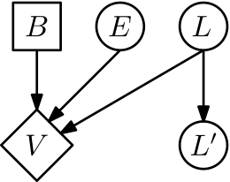
Here is an example for our setup: consider that we can ask an expert to provide us an estimate $L'$ of what the lowest bid $L$ could be.

Expert advice

By assuming a probability model $P(L' | L)$ we can relate the true unknown lowest bid $L$ to the experts guess.

The influence diagram looks as follows:

Influence diagram for the construction company with expert advice

Recipe for Value of Information Computation

To understand how the above derivation extends to this case, let us state a recipe of computing value of information:

State the expected utility, conditioned on decisions and the information to be valued.
Maximize the expression of step 1 over all decisions.
Marginalize the expression of step 2 over the information to be valued, using your prior beliefs. The resulting expression is the expected utility with information.
Start over: state the expected utility, conditioned only on decisions.
Maximize the expression of step 4 over all decisions. The resulting expression is the expected utility without information.
Compute the value of information as the difference between the two expected utilities (step 3 minus step 5).

This recipe works for any single-step decision problem, and any potential difficulties are computational.

Application of the Recipe to our Example

Here is its application to our generalized example:

This is $\mathbb{E}[V | L', B]$ which is obtained by marginalizing over $E$ and $L$ in $\mathbb{E}[V | L', B, E, L]$ and the marginal of $L$ is $P(L|L')$ obtained by Bayes rule.
Maximize over $B$, obtaining $\max_B \mathbb{E}[V | L', B]$.
Take the expectation over $L'$, which is defined via $P(L') = \mathbb{E}_{L}[P(L'|L)]$, yielding
\begin{equation} \mathbb{E}_{L'}[\max_B \mathbb{E}[V | L', B]]\label{eqn:Ltick-withinfo} \end{equation}
This is $\mathbb{E}[V | B]$ which is obtained by marginalizing over $E$ and $L$, here the marginal of $L$ is the prior $P(L)$.
Maximize over $B$, obtaining
\begin{equation} \max_B \mathbb{E}[V | B].\label{eqn:Ltick-withoutinfo} \end{equation}
The value of information is the difference between (\ref{eqn:Ltick-withinfo}) and (\ref{eqn:Ltick-withoutinfo}),
$$ \textrm{EVPI}(L') = \mathbb{E}_{L'}[\max_B \mathbb{E}[V | L', B]] - \max_B \mathbb{E}[V | B].$$

To make the above example concrete, let us assume that our expert is unbiased and we have

$$P(L'|L) = \mathcal{N}(L, \sigma),$$

where $\sigma > 0$ is the standard deviation. Computing $\textrm{EVPI}(L')$ as a function of $\sigma$ is possible by solving the maximization and integration problems.

Using the same parameters as before and using Monte Carlo for the integration, here is a visualization of the fair price to pay our expert.

Price for expert advice as a function of expert reliability

We can see that for $\sigma \to 0$ we recover the previous case of perfect information as the expert provides increasingly accurate knowledge about $L$ when $\sigma$ decreases. Conversely, with increasing expert uncertainty the value of his expert advice decreases.

Computation

(This was added in April 2016 after the original article was published.)

Computing the EVPI can be challenging because in many cases both the maximization problem and the expectation are intractable analytically and sample-based Monte Carlo approximations induce a non-negligible bias.

The recent work of (Takashi Goda, "Unbiased Monte Carlo estimation for the expected value of partial perfect information", arXiv:1604.01120) addresses part of the computation diffulties by application of a randomly truncated series to de-bias the ordinary Monte Carlo estimate. I have not performed any experiments but it seems to be a potentially useful method in the context of value of information computation problems.

Summary

From a formal decision theory point of view the value of information does not occupy a special place. It just measures the difference between two different expected utilities, given optimal decisions.

But value of information appears frequently in almost any statistical decision task. Here are two more examples.

In active learning we are interested in minimizing the amount of supervision needed to learn to perform a task and we can obtain supervision (ground truth class labels, for example) for instances of our choice at a cost. By applying value of information we can select for supervision the instances whose revealed label information brings the highest expected increase in utility.

In experimental design we have to make choices about which information to acquire, such as the number of patients to sample in a medical trial, or what information to collect at different costs in a customer survey. Value of information provides a way to make these choices, both statically, or better, adaptively.

Limitations

While decision theory is rather uncontroversial, it is a normative theory, that is, it tells you how to derive decisions which are optimal and coherent (rational). There are two main limitations I would like to point out:

As a normative theory it cannot claim to be a description of how humans (or other intelligent agents) make decisions.
It assumes infinite reasoning resources on behalf of the acting agent.

Both limitations are related of course in that real intelligent agents may deviate from normative decision theory precisely because they are limited in their reasoning abilities. There are both normative and descriptive theories to address these limitations. On the normative side we have for example computational rationality, taking into account the computational costs of reasoning and deriving optimal decisions within these constraints. On the descriptive side we have for example prospect theory, aiming to describe human decision making.